How Do We Use Eigenvectors?
Using eigen-axes to model matrices
Topics Covered
- Case 1: Regular axes
- Case 2: Different axes (locked)
- Application: Fibonacci and The Golden Ratio (locked)
- Case 3: Eigen-axes that are not perpendicular (locked)
- Other Cases (locked)
In the previous page you saw that once we have an eigenvector, every vector on the same line through the origin is also an eigenvector with the same eigenvalue:
You also saw the different arrangements of eigen-axes available for a matrix. In this page, you will see how we use those eigen-axes to model what happens to every vector in .
Case 1: Regular axes
Eigen-axes are incredibly useful for modeling what matrices do to vectors. To see this clearly, we'll start with the very nice case where the eigen-axes are the -axis and -axis.
Eigen-axes are the regular axes
Scaling the coordinates by the eigenvalues gives a very natural way to model what the matrix is doing.
Example 1: and
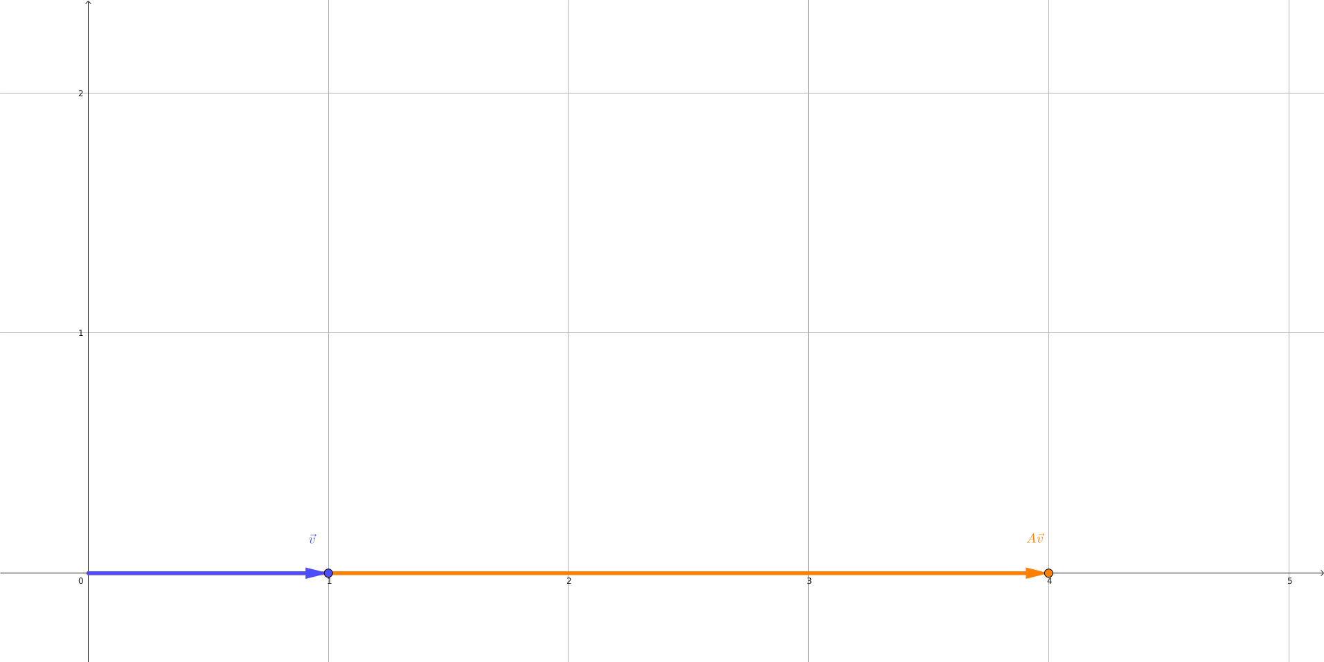
Example 2: and
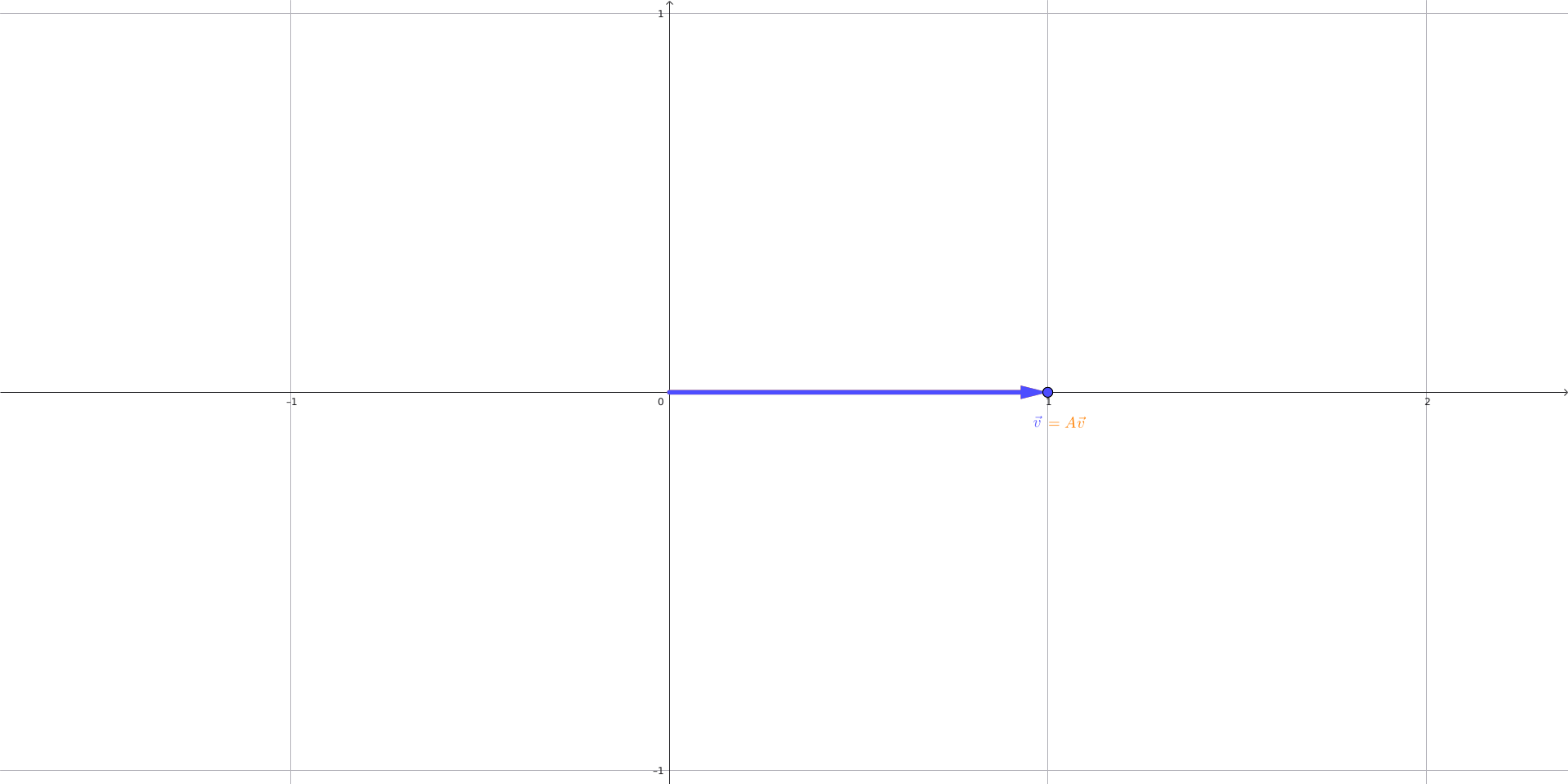
Example 3: Matrix powers, and
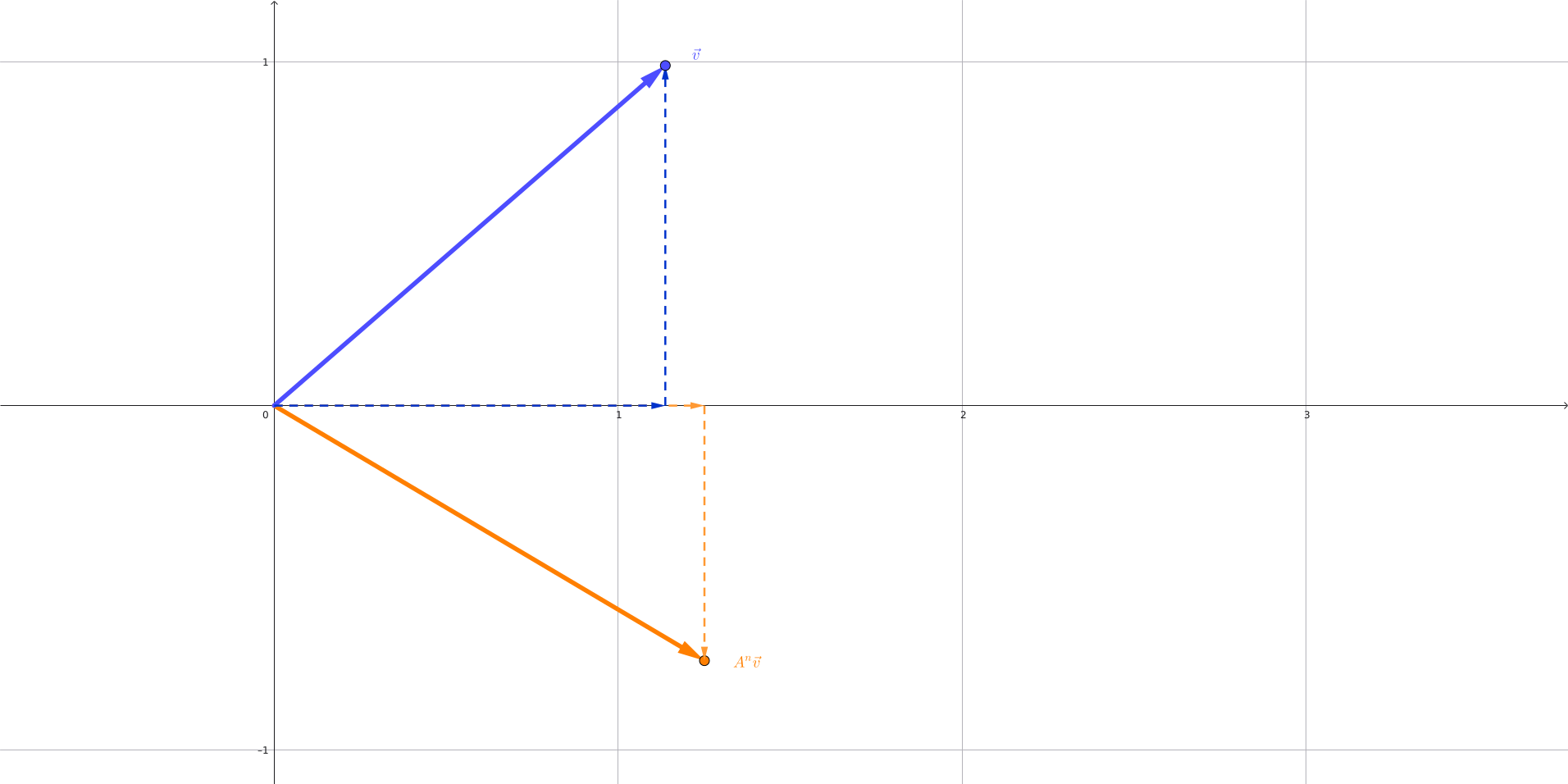
Problem 1: Using eigen-axes to model repeated applications of a matrix
If and for a matrix , what does do the vector ?
Answer Problem 1 correctly to reveal Case 2.